This post is again about improving the upsampling of the half-resolution SSAO render target used in the VKDF sponza demo that was written by Iago Toral. I am going to explain how I used information from the normals to understand if the samples of each 2×2 neighborhood we check during the upsampling belong to the same surface or not, and how this was useful in the upsampling improvement.
But before I start explaining these normal based samples classifications, a quick overview of our conclusions so far:
- In part 1 we’ve seen that the nearest depth algorithm from NVIDIA can reduce the artifacts where we have depth discontinuities but cannot improve significantly the overall upsampling quality.
- In part 2 we’ve seen that downsampling the z-buffer by taking the maximum sample of each 2×2 neighborhood or by taking once the minimum and once the maximum following a checkerboard pattern works well with the nearest depth but the overall quality is still very bad.
- In part 3.1 we’ve seen that it is possible to use different upscaling algorithms for the surfaces and the regions where we detect depth discontinuities. The idea was to use some sort of weighted average when all the samples of a neighborhood belong to the same surface and the nearest depth algorithm when we detect a depth discontinuity (not all samples belong to the same surface). We tried to classify the sample neighborhoods to “surface neighborhoods” and “discontinuity neighborhoods” using only depth information and we’ve seen that this is not working well as the method depends on what is visible on the screen and on the near and far clipping planes positions. But the idea to classify the pixels was very promising.
So, in this post, we are going to try the same classification, but this time using the normals instead of the depths for the reasons we have already explained in Post 3.1.
Using the normals to classify the samples
The idea is the following:
In the Vulkan pass that we downscaled the z-buffer (see post 1, post 2), we also downsample the normal buffer by selecting the sample that corresponds to the selected depth.
Then, in the upsampling pixel shader, we calculate the dot products between the normals of each 2×2 neighborhood of the downscaled normal buffer and we select the minimum among them. If its value is close to 1 we assume that the samples lie in the same surface and we perform linear interpolation. Otherwise, we assume that there is a discontinuity in the region and we perform nearest depth.
Why is this necessary?
Let’s see some basic maths:
The dot product of two normals a and b is calculated as:
|
1 |
a · b = |a| * |b| * cosθ |
where θ is the angle between the normals.
As the downsampled normals are already normalized at this point:
|
1 |
|a| * |b| = 1 |
the dot product equals the cosθ:
|
1 |
a · b = cosθ |
The equation above implies that:
- When the angle θ is small and the normal directions are almost parallel (like for example when the samples belong to the same surface) the dot product will take a value close to 1 (
cos0 = 1). - Also, if the minimum dot product between the normals of the neighborhood has a value close to 1.0 all the other dot products have also a value close to 1.0 and all the 4 normals are almost parallel to each other.
So when the minimum dot is ~1 we can safely assume that all the 4 samples lie in the same surface and we should average the colors to achieve a smooth result. In every other case, we can assume that there’s at least one normal with different direction and so there is at least one sample that lies on an edge or on a corner or on a separate surface (depth discontinuity). In that case, it doesn’t make sense to average the colors as we will miss the change in depth, and so we should prefer the nearest depth in order to increase the probability to select the sample that is different from the others.
Let’s see how this algorithm is able to distinguish the edges from the surfaces. With a threshold of: 0.992 (again selected by trial and error) I’ve generated the following image where the surfaces are white and the depth discontinuities are black:
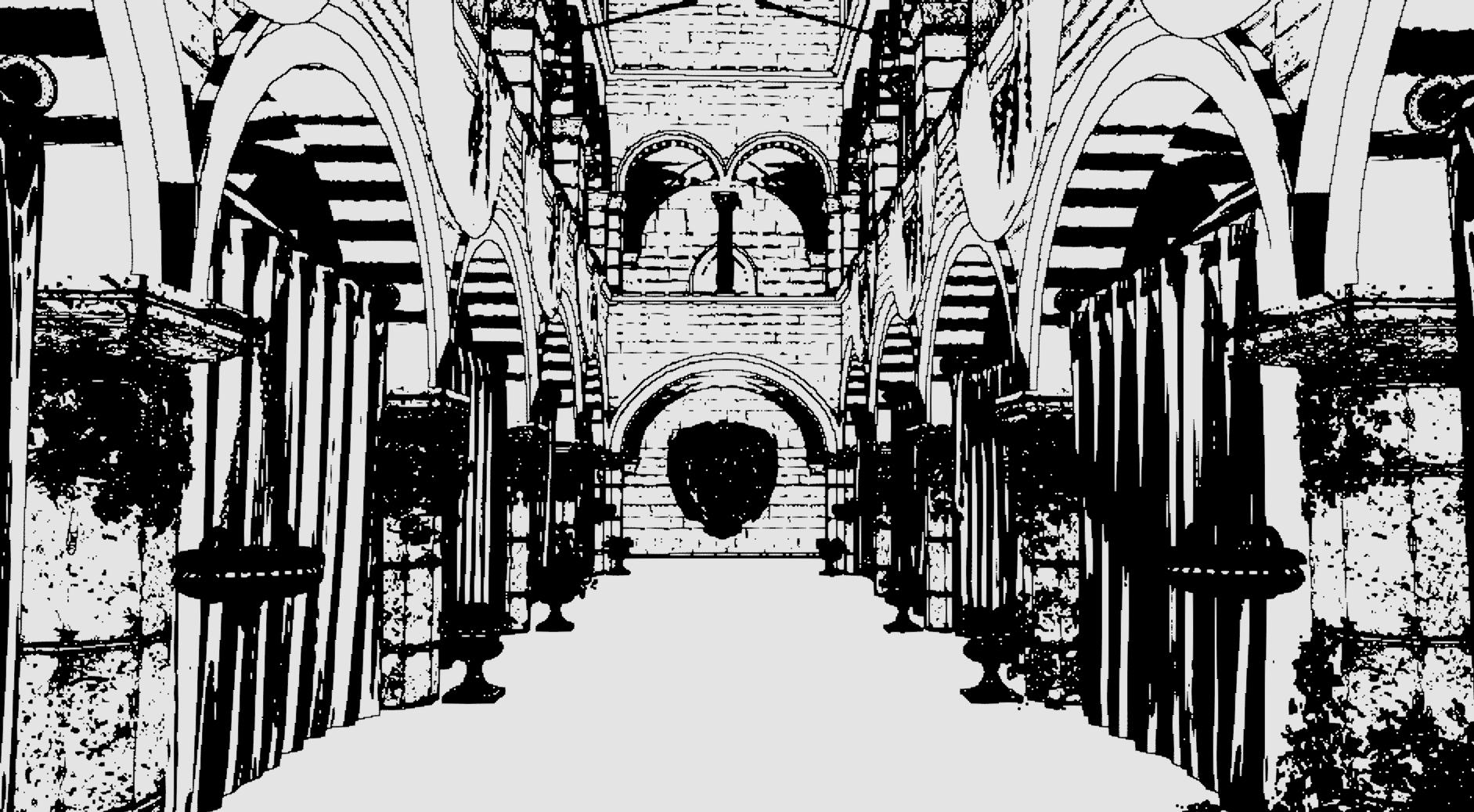
As the goal is to detect as many discontinuity points as possible (and not to achieve the best edge detection) I preferred to have more black regions in order to catch all the changes in depth than more white regions and accidentally ignore sudden depth changes.
As I already have explained in the previous post this “edge-detection”-like result is not dependent on the visible part of the scene at the time I selected the threshold and it does not depend on parameters like the near/far clipping planes positions. Therefore, we can achieve similar results in other scenes, when we move the camera and when we navigate around.
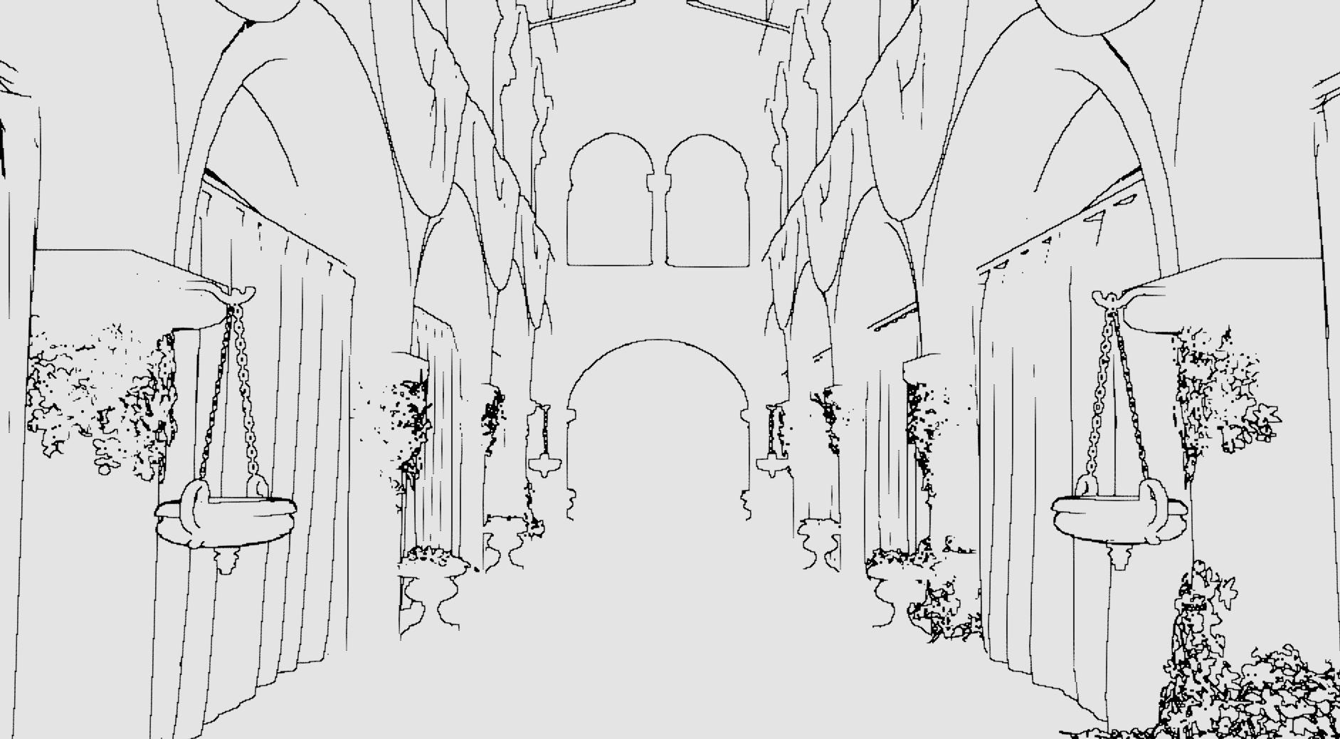
Using the normal to classify the sample neighborhoods to “surface neighborhoods” and “discontinuities neighborhoods” seems to give far better results than using the depth to perform the classification (click on the images below for comparison, the first is the normal-based classification whereas the second is the depth-based one from my previous post):
Some Code
Let’s first see how the algorithm described above would look in GLSL:
|
1 2 3 4 5 6 7 8 9 10 11 12 13 14 15 16 17 18 |
/* 2x2 neighborhood normals */ vec3 n0 = textureOffset(low_normal_tex, in_uv, ivec2(0, 0)).xyz; vec3 n1 = textureOffset(low_normal_tex, in_uv, ivec2(0, 1)).xyz; vec3 n2 = textureOffset(low_normal_tex, in_uv, ivec2(1, 0)).xyz; vec3 n3 = textureOffset(low_normal_tex, in_uv, ivec2(1, 1)).xyz; /* we need to find the minimum dot product */ float d0 = dot(n0, n1); float d1 = dot(n0, n2); float d2 = dot(n0, n3); float min_dot = min(d0, min(d1, d2)); float selection = step(0.992, min_dot); float lerp_occlusion = texture(ssao_tex, in_uv).x; float best_depth_occlusion = nearest_depth_occlusion(ssao_tex_nearest, depth_tex, low_depth_tex, in_uv); return mix(best_depth_occlusion, lerp_occlusion, selection); |
Note: In order to sample the SSAO render target once with the GLSL texture function (and perform linear interpolation) and once with the textureOffset (but this time without any filtering as I am doing the upsampling myself by performing nearest depth) I needed two samplers for the same texture in the shader. The first (the ssao_tex sampler2D) was created with VK_FILTER_LINEAR whereas the second (the ssao_tex_nearest) was created using the VK_FILTER_NEAREST. (There can probably be other ways to do the same thing, for example texelFetch doesn’t do any filtering but I prefered to use 2 samplers and keep things simple).
Vulkan side:
At this point (that I was trying to find a method to improve the upscaling quality) I didn’t care much about performance and optimizations, I only cared about reducing the artifacts. Therefore, I just added an extra color attachment to the Vulkan pass that downscales the Z-buffer in order to downsample the normals. Later, when I finally found a method that could significantly reduce the artifacts (future post), I decided to optimize things a little and pack the depths and the normals in the alpha and rgb values of the color attachment respectively instead of using 2 attachments.
So, in this Vulkan pass, I used as inputs the full-resolution depth and normal textures. The outputs were the downscaled normals of the selected samples in a color texture and the downscaled depths in a depth texture. I then used the downscaled outputs as inputs in the lighting pass and used them to upscale the SSAO texture.
The parameters I used for the color attachment of the depths/normals resize pass (just for symmetry with Part 1 where I shared the ones for the depth attachment) were:
– render target:
|
1 2 3 4 5 6 7 8 9 |
VK_IMAGE_TYPE_2D, VK_FORMAT_R16G16B16A16_SFLOAT, VK_FORMAT_FEATURE_COLOR_ATTACHMENT_BIT | VK_FORMAT_FEATURE_SAMPLED_IMAGE_BIT, VK_IMAGE_USAGE_COLOR_ATTACHMENT_BIT, VK_IMAGE_USAGE_SAMPLED_BIT, VK_MEMORY_PROPERTY_DEVICE_LOCAL_BIT, VK_IMAGE_ASPECT_COLOR_BIT, VK_IMAGE_VIEW_TYPE_2D |
– some render pass options for the normals buffer attachment (size was the size of the SSAO render target):
|
1 2 3 4 5 |
VK_FORMAT_R16G16B16A16_SFLOAT, VK_ATTACHMENT_LOAD_OP_DONT_CARE, VK_ATTACHMENT_STORE_OP_STORE, VK_IMAGE_LAYOUT_UNDEFINED, VK_IMAGE_LAYOUT_COLOR_ATTACHMENT_OPTIMAL, |
– color image sampler layout:
|
1 |
VK_IMAGE_LAYOUT_SHADER_READ_ONLY_OPTIMAL |
As I said I could have packed the depths and the normals in one color attachment. In that case I would still use the same parameters I used above for the attachment.
The downsampling part:
|
1 2 3 4 5 6 7 8 9 10 11 12 13 14 15 16 17 18 19 20 |
float depths[] = float[] ( textureOffset(tex_depth, in_uv, ivec2(0, 0)).x, textureOffset(tex_depth, in_uv, ivec2(0, 1)).x, textureOffset(tex_depth, in_uv, ivec2(1, 1)).x, textureOffset(tex_depth, in_uv, ivec2(1, 0)).x); vec3 normals[] = vec3[] ( textureOffset(tex_normal, in_uv, ivec2(0, 0)).xyz, textureOffset(tex_normal, in_uv, ivec2(0, 1)).xyz, textureOffset(tex_normal, in_uv, ivec2(1, 1)).xyz, textureOffset(tex_normal, in_uv, ivec2(1, 0)).xyz); max_depth = max(max(depths[0], depths[1]), max(depths[2], depths[3])); for (int i = 0; i < 4; i++) { if (max_depth == depths[i]) { normal = normals[i]; break; } } |
where tex_depth is the original (high resolution) depth buffer and tex_normal the original (high resolution) normal buffer.
Note: In the snippet above, I used the maximum depth of the neighborhood, but I could have used the checkerboard pattern we’ve seen in Part 2 of the series. The result was similar and you can see videos of both in the playlist I will append at the end of this post.
An attempt to avoid the downsampling and select normals from the high resolution normal buffer using offsets:
One thing I wanted to investigate was if I could avoid the downscaling of the normal buffer somehow. My idea was to select some normals from the original normal-buffer in offsets calculated by taking the SSAO scale into account. That could be easy as the full-resolution normal buffer was already available in the pixel shader where we performed the upscaling and the lighting, as part of the gbuffer textures that were used in the deferred shading calculations, see again Iago’s post.
So my first (naive) approach was to select 4 samples in a distance that depends on the scale around each sample (the downsampling was the same as in Part 1, Part 2, a pass that downscales the z-buffer):
|
1 2 3 4 |
vec3 n0 = texture(normal_tex, in_uv + ivec2(0, 0)).xyz; vec3 n1 = texture(normal_tex, in_uv + ivec2(0, int(SSAO_DOWNSAMPLING))).xyz; vec3 n2 = texture(normal_tex, in_uv + ivec2(int(SSAO_DOWNSAMPLING), 0)).xyz; vec3 n3 = texture(normal_tex, in_uv + ivec2(int(SSAO_DOWNSAMPLING), int(SSAO_DOWNSAMPLING))).xyz; |
where SSAO_DOWNSAMPLING is a specialization constant that depends on the SSAO resolution: in half resolution it’s 2.0, in 1/4 resolution it’s 4.0 and so on. I could perfectly have used a push constant, but I wanted to be able to use it with textureOffset as well, so I preferred the specialization.
I somehow expected that the quality wouldn’t be the same as with the downscaled normal buffer as these normal samples won’t be exactly the ones that correspond to the selected depth samples of the low resolution z-buffer but some neighboring ones. I was hoping though that it would give an acceptable result, especially where the discontinuities aren’t too many (surfaces) and the normals of the neighborhood are almost parallel. There would certainly be some artifacts caused by normals that don’t match the depth samples in some neighborhoods but hopefully the overall quality would be close to the quality I achieved with the normal buffer downsampling.
But this didn’t happen. 🙂 The classification result was really disappointing. There were too many artifacts, the discontinuity detection was varying depending on what was visible on the screen and sometimes it was dismissing whole surfaces (like the floor).
It was like the selected normals were random. And actually they were… And in order to select the normal that corresponds to the selected depth using offsets I would need a more complex shader:
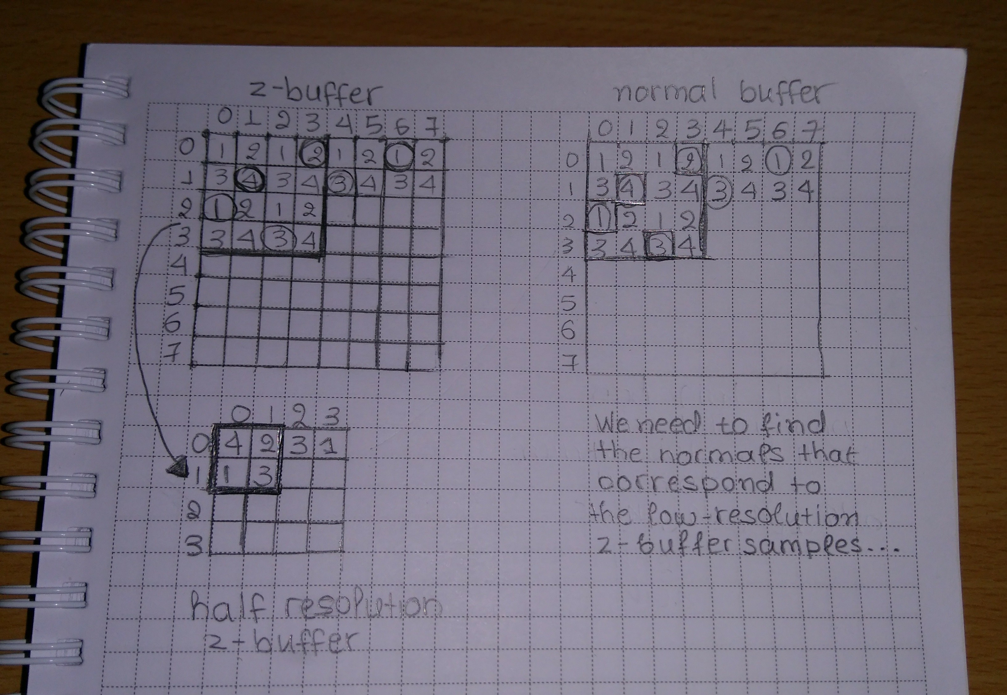
In the image above, on the left we see the z-buffer and the half-resolution z-buffer (suppposing that we perform SSAO in 1/2 resolution). Our downscaling algorithms so far (see part 1, part 2), select either the maximum or the minimum or both following some pattern like the checkerboard. Supposing that the circled samples of the z-buffer are the selected ones, the downsampled z-buffer contains a different sample of each 2×2 neighborhood of the original in each position: the one that is the max or the min depending on the pattern.
So, in order to find the normal that corresponds to that sample in the original normal buffer (the circled samples on the right) we would need to perform a similar depth comparison in the original depth buffer for each neighborhood of each sample. Then after having calculated the offsets and selected the normals N(3, 0), N(1, 1), N(0, 2) and N(2, 3) of the normal buffer, we would have to calculate their dots and select the minimum among them. This is already quite complex, similar to the downsampling we have already performed, and the complexity to select the correct sample increases while we lower the SSAO resolution and we change the radius of our search. So, at the end it’s faster and easier to just downscale the normal buffer.
I didn’t try to tweak this method further and see if I can select better offsets etc as it didn’t seem to have any significant performance advantage and the normal buffer downscaling clearly works.
And a note to myself: Replace that photo above with a proper diagram one day… :-p
Visual results
So is that method really an improvement?
Well, with this method we certainly reduced the sharp artifacts and misplacements we’ve seen that a depth-based classification can cause (part 3.1). Also, it is an improvement compared to the depth-aware alone and to lerp alone. But there are still visible artifacts in 1/2 resolution (videos), so there must still be room for improvement.
In the images (1/4 resolution) and the videos (1/2 resolution) below, we can see some comparisons of combinations of lerp in the surfaces with nearest depth where we spot discontinuities.
Max depth/Nearest depth vs Max depth/Nearest depth where we have discontinuities and Lerp on the surfaces:


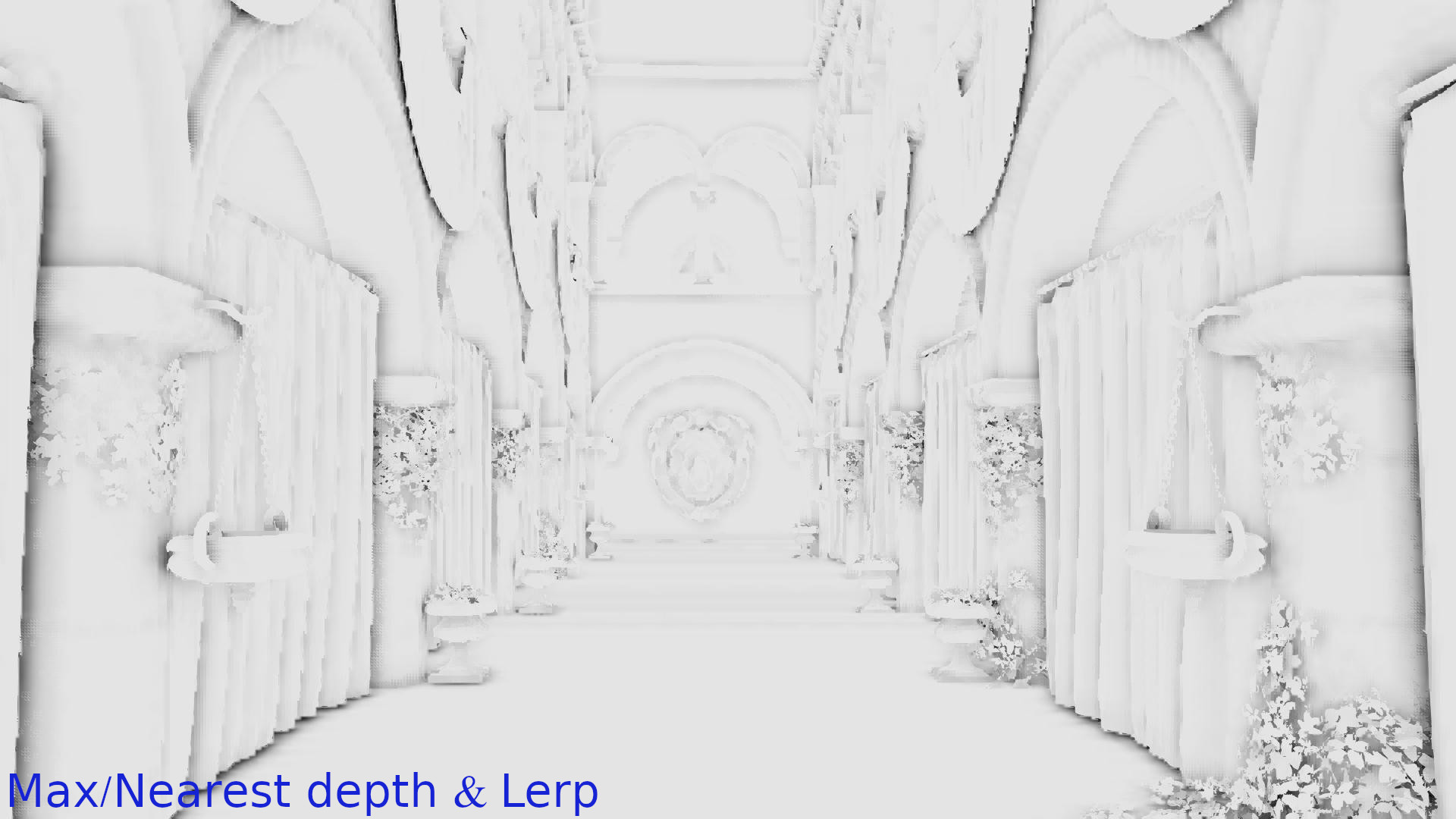
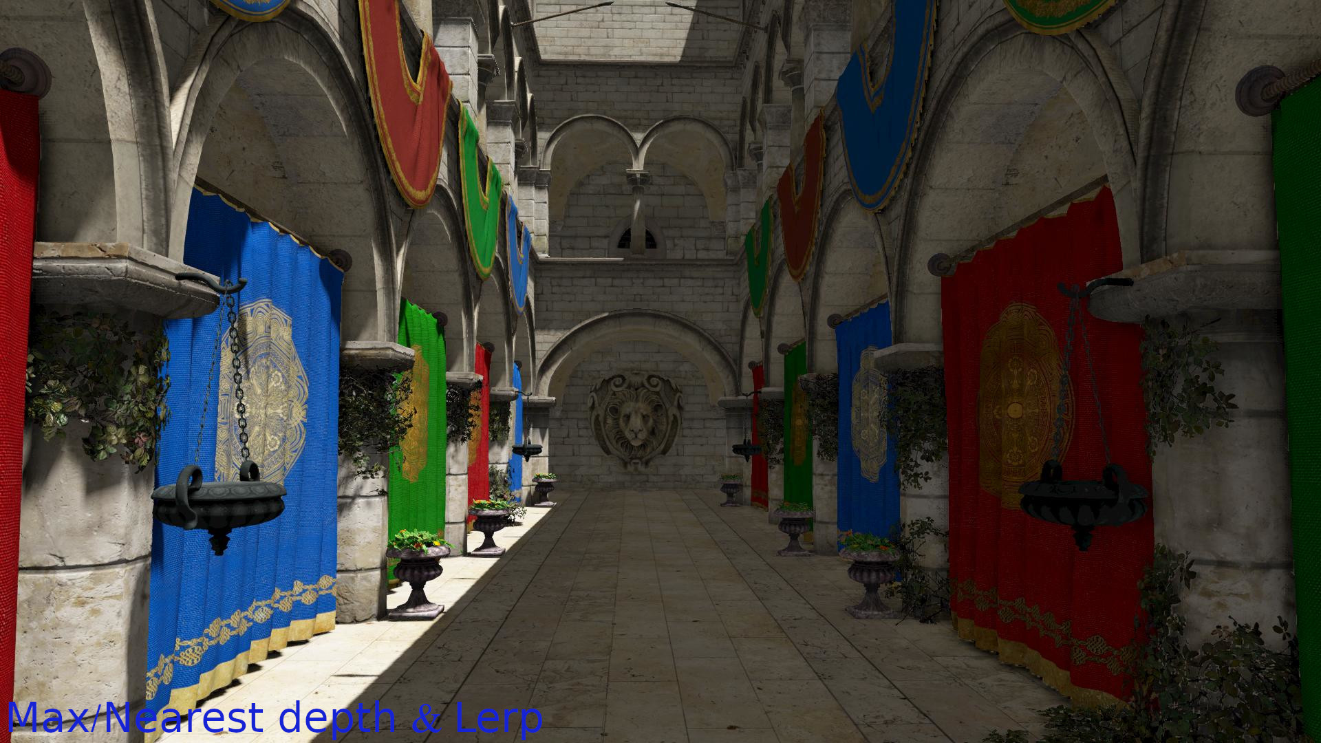
The Max depth/Nearest depth and lerp seems to be an improvement here. Although there are still some visible artifacts.
Checkerboard/Nearest depth vs Checkerboard/Nearest depth where we have discontinuities and Lerp on the surfaces:
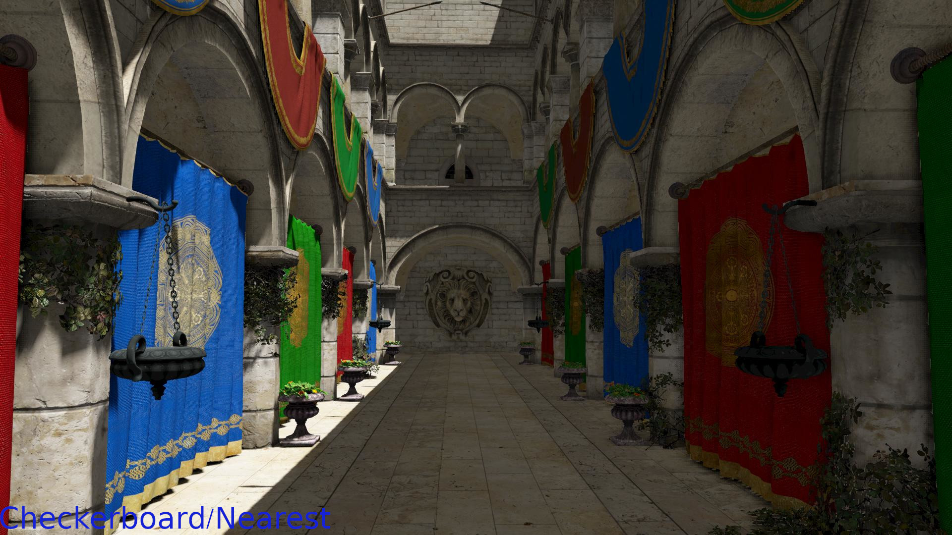
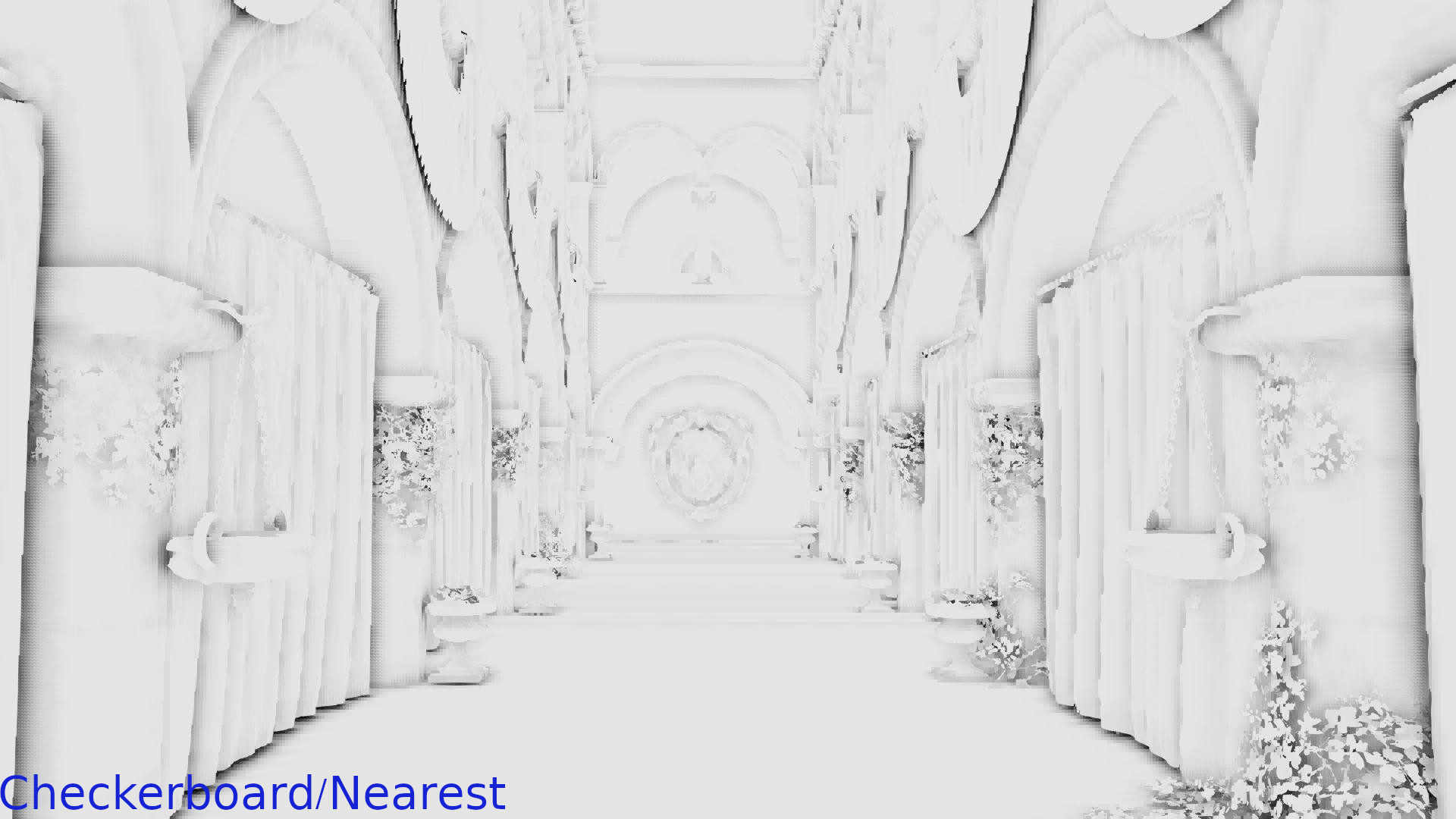
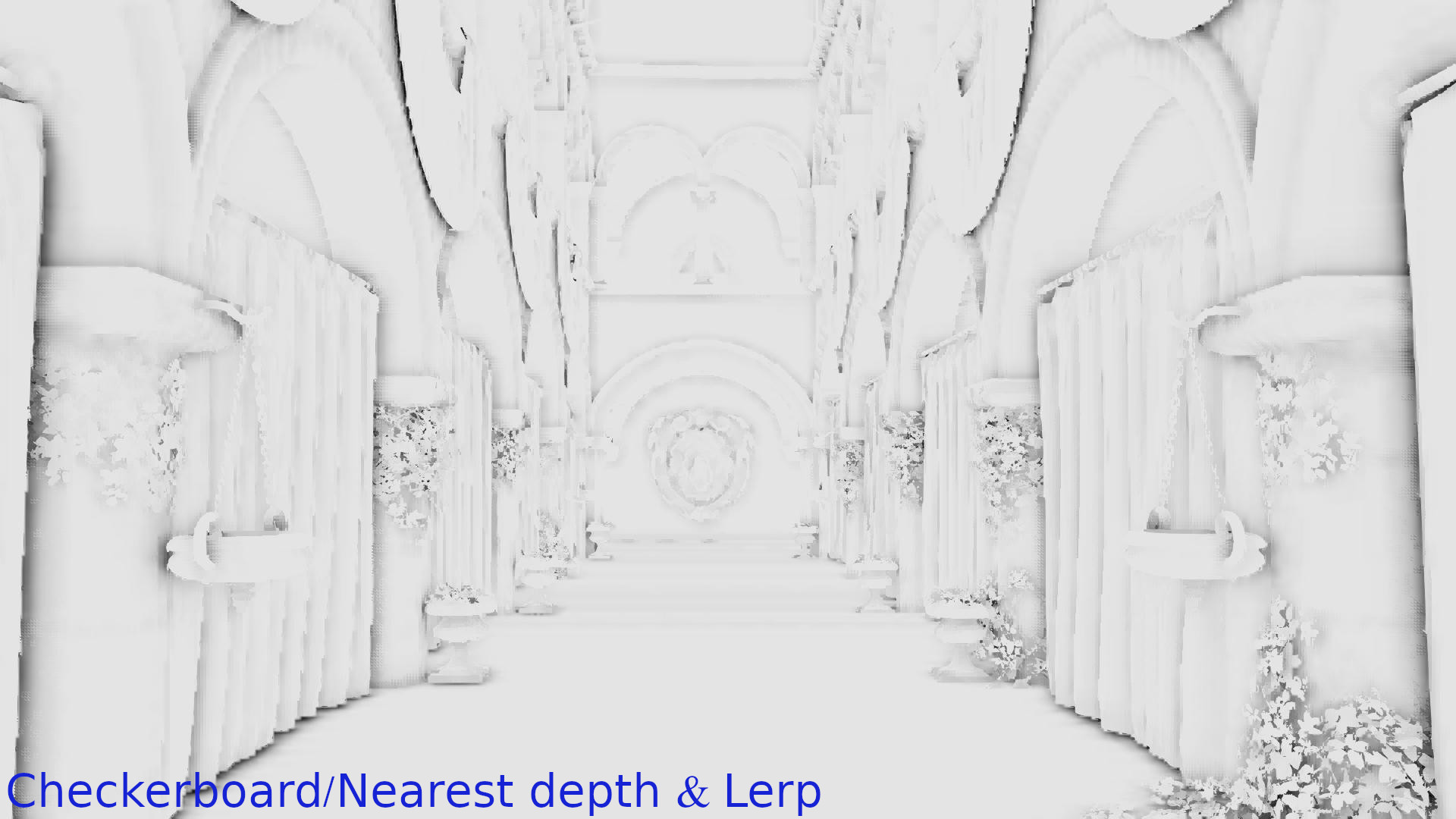

Same as above.
Max depth/Nearest depth where we have discontinuities and Lerp on the surfaces vs Checkerboard/Nearest depth where we have discontinuities and Lerp on the surfaces:
Here, the methods seem almost identical… So, I would use the less expensive if I really cared about performance (max depth). If the difference in FPS is small (future post) I would probably prefer the checkerboard because in theory it preserves more information.
Conclusions
So far, my conclusions were the following:
- Using the normal from a normal buffer downscaled with the exact same algorithm that we used to downscale the depth buffer works very well in distinguishing “surface neighborhoods” from “neighborhoods with depth discontinuities”.
- Using linear interpolation on the surfaces and nearest depth in the discontinuities improves a lot the result but maybe there is still room for improvements.
- Using the maximum depth or using once the minimum and once the maximum depth following a checkerboard pattern in the z-buffer/normal-buffer downsampling step doesn’t make a significant difference: checkerboard makes more sense but we could easily replace it with the maximum depth that is simpler and depending on how we implement the checkerboard maybe less expensive too.
Also, although there is still room for improvement and we can try to further reduce the artifacts (next post), the SSAO using Lerp on surfaces and Nearest depth on discontinuities is probably acceptable too:
To sum up:
In this post, we’ve seen that:
- We can successfully use the normals to classify the 2×2 neighborhoods of the SSAO texture in neighborhoods that contain depth discontinuities and in neighborhoods where all the samples belong to the same surface.
- There are 2 different ways to achieve the classification: we can either downsample the normal buffer or calculate offsets in the original normal buffer but the latter is expensive and complex if we want to do it properly so we prefer the downsampling.
- There is no significant difference between downsampling with checkerboard or using max depth. Selecting the maximum is less expensive but checkerboard makes more sense as in theory it preserves more depth information.
- Although we are getting close to achieve a good result, there might still be room for improvement especially in lower resolutions.
Next post
In the next post of the series, I will talk about other ideas to improve the quality and compare them with the current one. I will also try to do some performance comparisons and see if reducing resources can further optimize the SSAO.
Closing:
Like in the previous posts, I am appending the playlist with the videos used in the comparisons above in 1920×1080 resolution (SSAO is performed in 960×540) for those who want to examine the artifacts and the differences in detail: