| Home |
| Projects |
| Curriculum Vitae |
| Contact |
|
A path tracer, written in C++ for my "Advanced Modelling, Rendering and Animation"
assignment at UCL.
I based the code on a previous ray tracer
I wrote from scratch for another assignment some months before the path tracer that was using
the SDL library to present the pixels to the
user.
The program reads a text scene descriptor where all the object and light attributes are described and
renders the scene using the Path tracing algorithm.
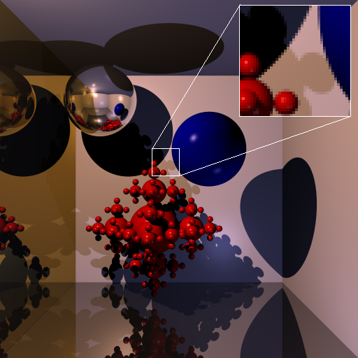
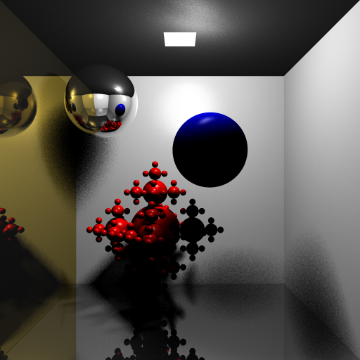
Path Tracing From Wikipedia: Path tracing is a computer graphics rendering technique that attempts to simulate the physical behaviour of light as closely as possible. It is a generalisation of conventional ray tracing, tracing rays from the virtual camera through several bounces on or through objects. The image quality provided by path tracing is usually superior to that of images produced using conventional rendering methods at the cost of much greater computation requirements. Path tracing naturally simulates many effects that have to be specifically added to other methods (conventional ray tracing or scanline rendering), such as soft shadows, depth of field, motion blur, caustics, ambient occlusion, and indirect lighting. Implementation of a renderer including these effects is correspondingly simpler. Due to its accuracy and unbiased nature, path tracing is used to generate reference images when testing the quality of other rendering algorithms. In order to get high quality images from path tracing, a large number of rays must be traced to avoid visible artifacts in the form of noise. More detailed references:[1] James T. Kasiya. The rendering equation. Computer Graphics, pages 143-150, 1986. [2] Eric P. F. Lafortune. Mathematical models and monte carlo algorithmics for physically based rendering. PHD thesis, Katholieke Universiteit Leuven, 1996. [3] James Arvo Marcos Fajardo Pat Hanrahan Henrik W. Jensen Don P. Mitchell Matt Phar Peter S. Shirley. State of the art in monte carlo ray tracing for realistic image synthesis. 2001. [4] Henrik W. Jensen. Importance driven path tracing using the photon map. Proc.6th Eurographics Workshop on Rendering, 1995. The project requirements explained step by step: Requirement 1: Many rays per pixel using stratification and jittering. The pixel is divided recursively to 4 subpixels according to the desired number of rays per pixel (this number is passed as a parameter and is rounded to a power of four). Then the center of each sub-pixel is randomly moved in an area between the boundaries of the sub-pixel.
Color avg_color(double pxl_width, double pxl_height, double x, double y, int depth) {
    Color c;
    double w = pxl_width;
    double h = pxl_height;

    if (depth == 0) {
        if(rays_ppxl > 1) {
            x += (double) rand() / RAND_MAX * pxl_width - pxl_width / 2.0;
            y += (double) rand() / RAND_MAX * pxl_height - pxl_height / 2.0;
        }
        Ray ray = scene.get_camera()->get_primary_ray(x, y);
        c = trace(ray, MAX_DEPTH);
        c.x = c.x > 1.0 ? 1.0 : c.x;
        c.y = c.y > 1.0 ? 1.0 : c.y;
        c.z = c.z > 1.0 ? 1.0 : c.z;
        return c;
    }
    c = c + avg_color(w/2, h/2, x + w/4, y + h/4, depth-1);
    c = c + avg_color(w/2, h/2, x + w/4, y - h/4, depth-1);
    c = c + avg_color(w/2, h/2, x - w/4, y + h/4, depth-1);
    c = c + avg_color(w/2, h/2, x - w/4, y - h/4, depth-1);
    c = c/4;
    return c;
}
Requirement 2: Use of spherical, triangular and quadrilateral area light sources. The path tracer (that at this moment is still a Monte Carlo ray tracer) supports spheres, sphere flakes, planes, meshes of quads and meshes of triangles. From those objects, the spheres, the triangle meshes and the quad meshes can be used also as area lights. Instead of sending a ray to a point light source and test if an object of interest is in shadow or not, now we use a random point in the surface of the area light. In case of the sphere area lights, points are generated in the bounding cube until one is found to be inside the sphere (rejection sampling). In case of the triangular meshes, a triangle of the mesh is chosen randomly. Then, a point inside this triangle is chosen by calculating random �, � and � barycentric coordinates between 0 and 1. If �, � and � have sum greater than one we reject the point (rejection sampling) otherwise we calculate its Cartesian coordinates. In case of quadrilateral meshes, a quad of the mesh is chosen at random and then a random point in that quad is generated. In order to generate a random point in a quad, a random linear combination of 2 vectors of 2 consecutive edges of the quad is used. 

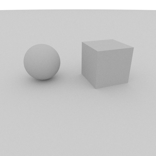
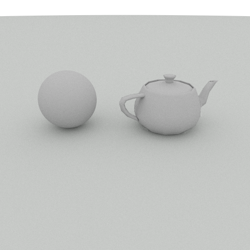
The same scene lit firstly by using a sphere area light, then by using a quad area light and then using a triangular mesh (teapot) area light. Vector3 Sphere::sample() const { double rndx, rndy, rndz; double magnitude; do { rndx = 2.0 * (double) rand() / RAND_MAX - 1.0; rndy = 2.0 * (double) rand() / RAND_MAX - 1.0; rndz = 2.0 * (double) rand() / RAND_MAX - 1.0; magnitude = sqrt(rndx * rndx + rndy * rndy + rndz * rndz); } while (magnitude > 1.0); Vector3 rnd_point(rndx / magnitude, rndy / magnitude, rndz / magnitude); return rnd_point * radius + center; } Vector3 Face::sample(MeshPrim prim) const { Vector3 smpl; if (prim == MESH_PRIM_TRI) { double a, b, c; do { a = (double) rand() / RAND_MAX; b = (double) rand() / RAND_MAX; c = (double) rand() / RAND_MAX; } while(a + b + c > 1.0); smpl = v[0].pos * a + v[1].pos * b + v[2].pos * c; } else { Vector3 edge_a = v[1].pos - v[0].pos; Vector3 edge_b = v[2].pos - v[0].pos; double a = (double) rand() / RAND_MAX; double b = (double) rand() / RAND_MAX; smpl = (a * edge_a) + (b * edge_b) + v[0].pos; } return smpl; } Requirement 3: Sampling the Lambertian and the Phong BRDFs. In case of specular surfaces the reflected ray directions form a lobe whereas in case of diffuse surfaces they are scattered in every direction in the hemisphere above the surface. In each case, a random vector was chosen inside the lobe or the hemisphere respectively and the probability to continue tracing or stop was calculated by evaluating the BRDF. In the pictures below, we can see the difference in the reflections of a sphere when sampling the Phong BRDF with various (decremented) specular exponents. 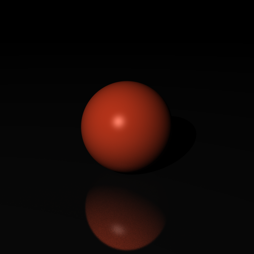
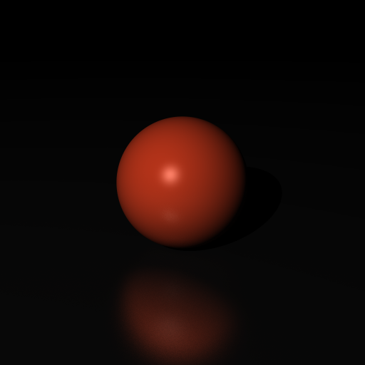
As the specular exponent is decreased the cone of directions is getting larger. Vector3 sample_phong(const Vector3 &outdir, const Vector3 &n, double specexp) { Matrix4x4 mat; Vector3 ldir = normalize(outdir); Vector3 ref = reflect(ldir, n); double ndotl = dot(ldir, n); if(1.0 - ndotl > EPSILON) { Vector3 ivec, kvec, jvec; // build orthonormal basis if(fabs(ndotl) < EPSILON) { kvec = -normalize(ldir); jvec = n; ivec = cross(jvec, kvec); } else { ivec = normalize(cross(ldir, ref)); jvec = ref; kvec = cross(ref, ivec); } mat.matrix[0][0] = ivec.x; mat.matrix[1][0] = ivec.y; mat.matrix[2][0] = ivec.z; mat.matrix[0][1] = jvec.x; mat.matrix[1][1] = jvec.y; mat.matrix[2][1] = jvec.z; mat.matrix[0][2] = kvec.x; mat.matrix[1][2] = kvec.y; mat.matrix[2][2] = kvec.z; } double rnd1 = (double)rand() / RAND_MAX; double rnd2 = (double)rand() / RAND_MAX; double phi = acos(pow(rnd1, 1.0 / (specexp + 1))); double theta = 2.0 * M_PI * rnd2; Vector3 v; v.x = cos(theta) * sin(phi); v.y = cos(phi); v.z = sin(theta) * sin(phi); v.transform(mat); return v; } Vector3 sample_lambert(const Vector3 &n) { double rndx, rndy, rndz; double magnitude; do { rndx = 2.0 * (double) rand() / RAND_MAX - 1.0; rndy = 2.0 * (double) rand() / RAND_MAX - 1.0; rndz = 2.0 * (double) rand() / RAND_MAX - 1.0; magnitude = sqrt(rndx * rndx + rndy * rndy + rndz * rndz); } while (magnitude > 1.0); Vector3 rnd_dir(rndx / magnitude, rndy / magnitude, rndz / magnitude); if (dot(rnd_dir, n) < 0) { return -rnd_dir; } return rnd_dir; } Requirement 4: BRDF evaluation. The formulas for the Phong and Lambertian models were used to evaluate the BRDF in case of specular and diffuse surfaces respectively. Case of diffuse interaction. double phong(const Vector3 &indir, const Vector3 &outdir, const Vector3 &n, double specexp) { Vector3 refindir = reflect(indir, n); double s = dot(refindir, outdir); if (s < 0.0) { return 0.0; } return pow(s, specexp); } double lambert(const Vector3 &indir, const Vector3 &n) { double d = dot(n, indir); if (d < 0.0) { d = 0.0; } return d; } Requirement 5: Put it all together to form paths that sample all the integrals. The path tracer sends many rays per pixel using stratification and jittering. Then, it traces each ray by calling recursively the shade function. In this function it samples each BRDF to decide if the tracing will continue or stop after a specific intersection. Requirement 6: Russian roulette (unbiased path termination). The method of Russian roulette was used to implement importance sampling. First, we decide if the next interaction will be diffuse or specular and second, we decide if the tracing will continue or not (unbiased path termination). In the first step, a random number is chosen between 1 and sum of the means of diffuse kd and the specular ks and if it is found larger than ks the next interaction is diffuse. Otherwise, it is specular. In the second step (unbiased path termination), the dot product of the randomly generated vector inside the lobe or the hemisphere (see previous requirement) with the normal of the surface is calculated and compared to the probability evaluated by the BRDF. If it is less or equal to the BRDF value the tracing continues otherwise it stops. /* russian roulette */ double avg_spec = (mat->ks.x + mat->ks.y + mat->ks.z) / 3; double avg_diff = (mat->kd.x + mat->kd.y + mat->kd.z) / 3; Vector3 newdir; double range = MAX(avg_spec + avg_diff, 1.0); double rnd = (double)rand() / RAND_MAX * range; if (rnd < avg_diff) { // diffuse interaction newdir = sample_lambert(n); if ((double) rand() / RAND_MAX <= lambert(newdir, n)) { Ray newray; newray.origin = p; newray.dir = newdir * RAY_MAG; color += trace(newray, depth - 1) * mat->kd / avg_diff; } } else if (rnd < avg_diff + avg_spec) { // specular interaction newdir = sample_phong(-ray.dir, n, mat->specexp); double pdf_spec = phong(newdir, -normalize(ray.dir), n, mat->specexp); if((double)rand() / RAND_MAX <= pdf_spec) { Ray newray; newray.origin = p; newray.dir = newdir * RAY_MAG; color += trace(newray, depth - 1) * mat->ks / avg_spec; } } Requirement 7: Create different scenes. Different scenes were created. 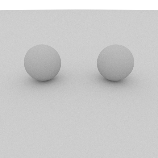


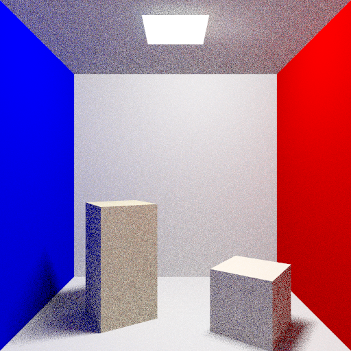


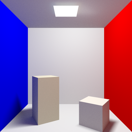
(1, 4, 16, 64, 256 and 1024 rays per pixel!) Other work: Some extra features were added to improve the result. For example, gamma correction was used to improve the appearence of the colors. 
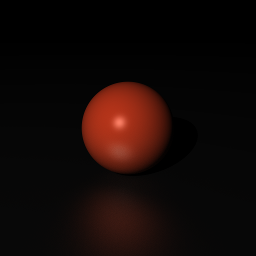
Full global illumination with gamma correction. The teapot used is a low polygon version of the Utah teapot. Download the Path Tracer and Run it: You can download the source code from here as well as a 32bit linux binary, a 64 bit linux binary, a windows executable or a mac os x binary. You can then run it or compile it according to the following README file:
To compile enter the directory path_tracer and type:
$ make

To run the program on Linux:
$./rt -parameter1 value1 -parameter2 value2 ...
(or ./rt-linux32 ./rt-linux64 if you are using the precompiled binaries)

Parameters:
-ray        integer for the number of rays
-gamma      gamma value (recommended value: 2.2)
-size       set the resolution (eg 256x256) - there is no aspect ratio support!
-nosdl      use this parameter if you don't want to use sdl (the picture will be
            saved in ppm format in file "out.ppm" of current directory.

Functional Keys:
"s" or "S"  save screenshot out.ppm in the current directory
Escape      exit the program

Mouse click on image points: prints the pixel coordinates (only for debug reasons)

To run the program on MacOSX:
$ ./rt-macosx64 -parameter1 value1 -parameter2 value2 ...
with same parameters as above.

To run the program on Windows:
rt-win32 -parameter1 value1 -parameter2 value2 ...
|